How safe are the websites of the cities of Italy?
Tempo di lettura: 6 minutiData pubblicazione: February 2, 2017
Disclaimer: The original post can be found here [Italian]
A few months ago I noticed that almost all of the municipal websites follow a common pattern, ie:
www.cityname.province.it
except for provincial capitals and other websites that have completely different domains. So I thought that I could scan with nmap all the sites of the cities of Italy, statistically analyzing the data with R and publishing the results.
List of websites
The list of sites is not available in text format. So I downloaded the list of the cities from the Istat website and wrote a script that follows the above pattern.
The number of websites today is 7983, while in my list there are 7161 sites, since, when scanning some were not reachable or were offline.
After I got the list of sites, I run nmap with the command:
nmap -sV -p 80,443 -O --script ssl-heartbleed --script http-enum --script-args 'http-enum.category="cms"' --script banner -iL ListofCities -oX ListofCities.xml
Data extraction
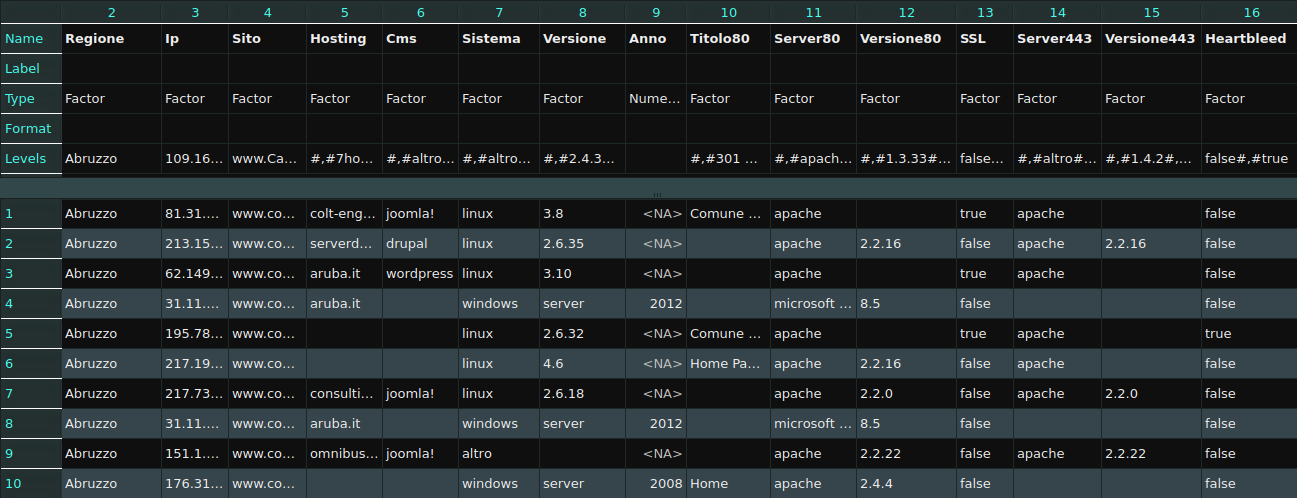
I didn’t find a specific parser for my purpose, so I wrote another script to parse the result. The script took a XML file and printed:
- IP address;
- Name of website;
- Hosting;
- Cms;
- Operating system (i’ve insert only Windows, Linux e Freebsd);
- Version of the operating system;
- Title, thanks to this class;
- Type of server on port 80;
- Version of server on port 80;
- Type of server on port 443;
- Version of server on port 443;
- Presence of SSL;
- Presence of vulnerability Heartbleed.
Data in R
The resulting file was uploaded on R, and I ran on it a series of commands, issued in the spoiler for those who want to better understand the graphics.
0.Upload file
args<-commandArgs(TRUE) Regione<-read.delim(args[1],sep=",",na.string=c("",NA)) cat(file=paste(args[1],".txt"),“Number of sites: “, nrow(Regione),sep="\n”) cat(“Su “,sum(table(Regione$Ip)),“host ci sono “,length(unique(Regione$Ip)),” indirizzi IP unici e il massimo possiede “,max(table(Regione$Ip)),” siti \n”,file=paste(args[1],“output”), append=TRUE)
1.Plot of Hosting
png(paste(args[1],“1Hosting.png”), units=“in”, width=11, height=8.5, res=300) op <- par(mar = c(0,17,4,2) + 0.1) barplot(sort(prop.table(table(Regione$Hosting))*100),horiz=TRUE,las=1,space=1,col=rainbow(length(table(Regione$Hosting))),names=paste(names(sort(prop.table(table(Regione$Hosting))*100)),"-",signif(sort(prop.table(table(Regione$Hosting))*100),2),"%"),main=paste(“Hosting utilizzato su”,sum(table(Regione$Hosting)),“host”),axes=FALSE)
2.Plot of Operating system
percentlabelsSIS pielabelsSIS png(paste(args[1],“2SistemiOP.png”), width=700, height=700, res=75) pie(prop.table(table(Regione$Sistema)),main=paste(“Sistemi operativi su”,sum(table(Regione$Sistema)),“host”),col=rainbow(length(table(Regione$Sistema))),labels=pielabelsSIS) legend(“topright”,legend=levels(Regione$Sistema),cex=0.8,fill=rainbow(length(table(Regione$Sistema))))
3.Plot of Windows versions
png(paste(args[1],“3VersioniWindows.png”),width=700, height=500, res=75) barplot(table(Regione[Regione$Sistema==“windows”,“Anno”]),col=rainbow(length(table(Regione$Anno))),main=paste(“Versioni di Windows su”,sum(table(Regione[Regione$Sistema==“windows”,“Anno”])),“host”),ylab=“Numero di host”,xlab=“Anno”)
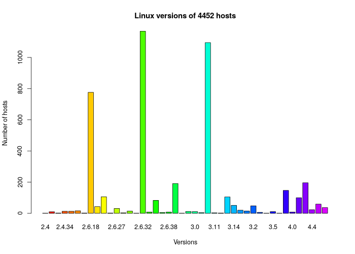
4.Plot of Linux versions
png(paste(args[1],“4VersioniLinux.png”), width=700, height=500, res=75) barplot(table(droplevels(sort(Regione[Regione$Sistema==“linux”,“Versione”]))),main=paste(“Versioni di linux su”,sum(table(droplevels(Regione[Regione$Sistema==“linux”,“Versione”]))),“host”),col=rainbow(length(table(Regione$Versione))),xlab=“Versione”,ylab=“Numero di host”)
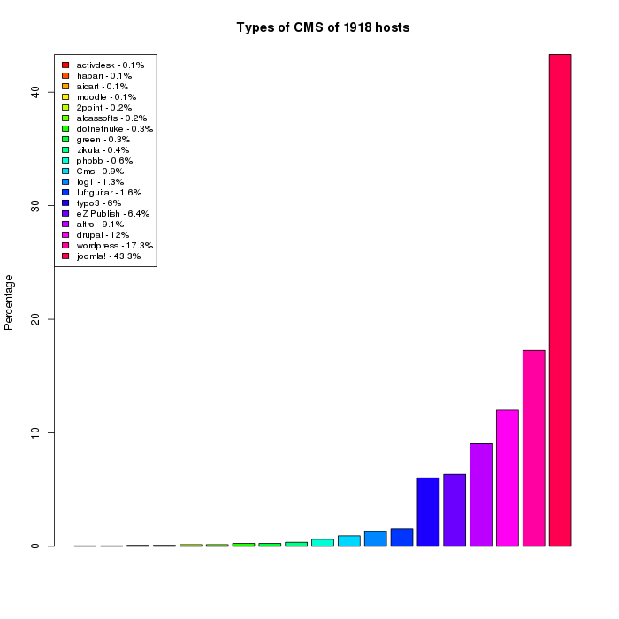
5.Plot of CMS
percentlabelsCMS pielabelsCMS png(paste(args[1],“5CMS.png”),width=700, height=700, res=75) pie(prop.table(table(Regione$Cms)),main=paste(“Tipi di Cms di”,sum(table(Regione$Cms)),“host”),col=rainbow(length(table(Regione$Cms))),labels=pielabelsCMS) legend(“topright”,legend=levels(Regione$Cms),cex=0.8,fill=rainbow(length(table(Regione$Cms))))
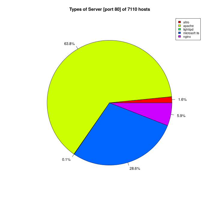
6.Plot of Server
percentlabelsSER80 pielabelsSER80 png(paste(args[1],“6TipidiServer80.png”), width=700, height=700, res=75) pie(prop.table(table(Regione$Server80)),main=paste(“Tipologie di Server [porta 80] su”,sum(table(Regione$Server80)),“host”),col=rainbow(length(table(Regione$Server80))),labels=pielabelsSER80) legend(“topright”,legend=levels(Regione$Server80),cex=0.8,fill=rainbow(length(table(Regione$Server80))))
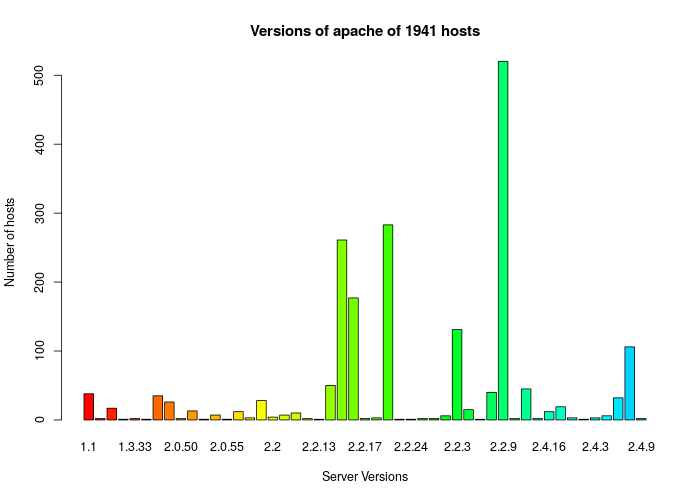
7.Plot of the version of Server
png(paste(args[1],“7MaxServer80Versioni.png”),width=700, height=500, res=75) barplot(table(droplevels(Regione[Regione$Server80==Regione[sum(table(Regione$Server80)),“Server80”],“Versione80”])),main=paste(“Versioni di”,Regione[sum(table(Regione$Server80)),“Server80”],“su”,sum(table(droplevels(Regione[Regione$Server80==Regione[sum(table(Regione$Server80)),“Server80”],“Versione80”]))), “host”) ,col=rainbow(length(table(Regione$Versione80))),xlab=“Versione server”,ylab=“Numero di host”)
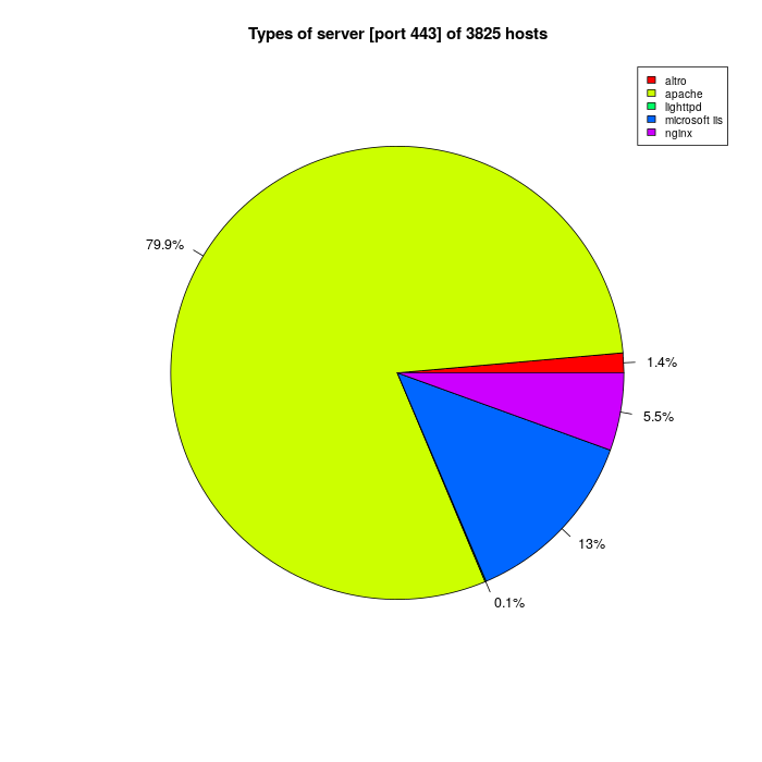
8.Plot of Server [443]
percentlabelsSER443 pielabelsSER443 png(paste(args[1],“8TipidiServer443.png”), width=700, height=700, res=75) pie(prop.table(table(Regione$Server443)),main=paste(“Tipologie di Server [porta 443] su”,sum(table(Regione$Server443)),“host”),col=rainbow(length(table(Regione$Server443))),labels=pielabelsSER443) legend(“topright”,legend=levels(Regione$Server443),cex=0.8,fill=rainbow(length(table(Regione$Server443))))
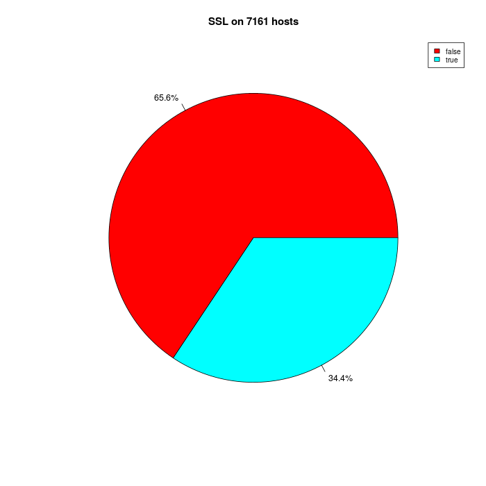
9.Plot of presence of SSL
percentlabelsSSL pielabelsSSL png(paste(args[1],“9SSL.png”), width=700, height=700, res=75) pie(prop.table(table(Regione$SSL)),main=paste(“Presenza di SSL su”,sum(table(Regione$SSL)),“host”),col=rainbow(length(table(Regione$SSL))),labels=pielabelsSSL) legend(“topright”,legend=levels(Regione$SSL),cex=0.8,fill=rainbow(length(table(Regione$SSL))))
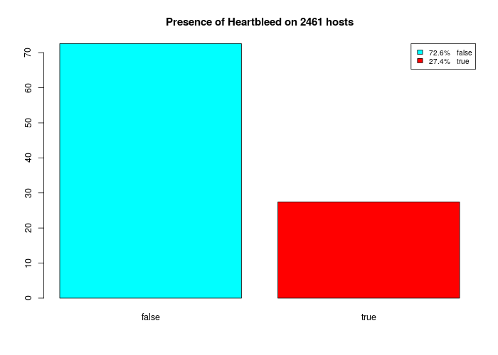
10.Plot of HeartBleed
percentlabelsHEA pielabelsHEA png(paste(args[1],“10Heartbleed.png”), width=700, height=500, res=75) barplot(prop.table(table(Regione[Regione$SSL==“true”,“Heartbleed”]))*100,main=paste(“Presenza vulnerabilità ad Heartbleed su”,sum(table(Regione[Regione$SSL==“true”,“Heartbleed”])),“host”),col=rev(rainbow(length(table(Regione[Regione$SSL==“true”,“Heartbleed”]))))) legend(“topright”,legend=paste(pielabelsHEA,” “,levels(Regione[Regione$SSL==“true”,“Heartbleed”])),cex=0.8,fill=rev(rainbow(length(table(Regione[Regione$SSL==“true”,“Heartbleed”])))))
Results
Number of cities: 7983
Number of analyzed hosts: 7161
Information of IP addresses: On 7161 hosts there are 2083 unique IP address. One of them maintains 779 websites
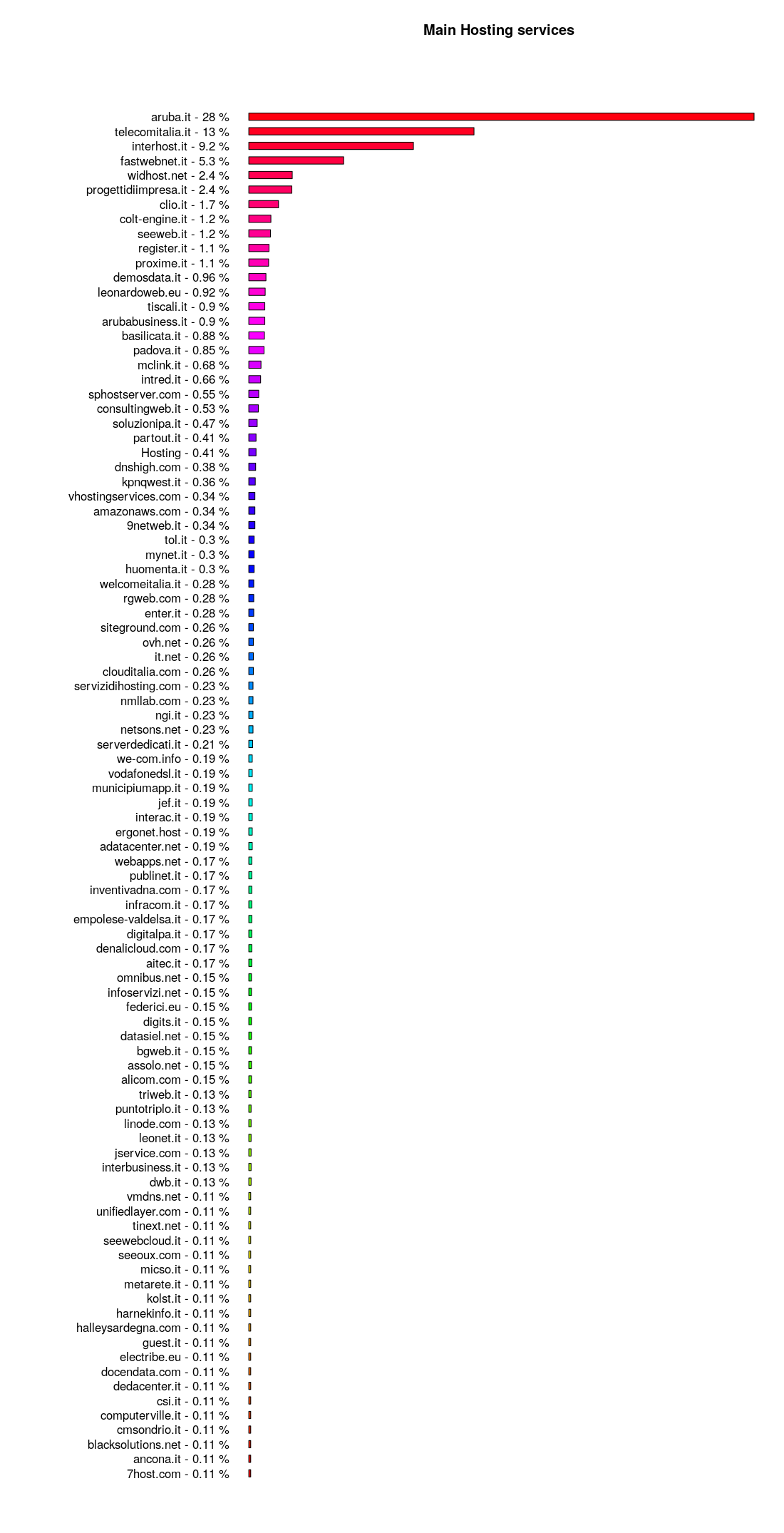
Hosting
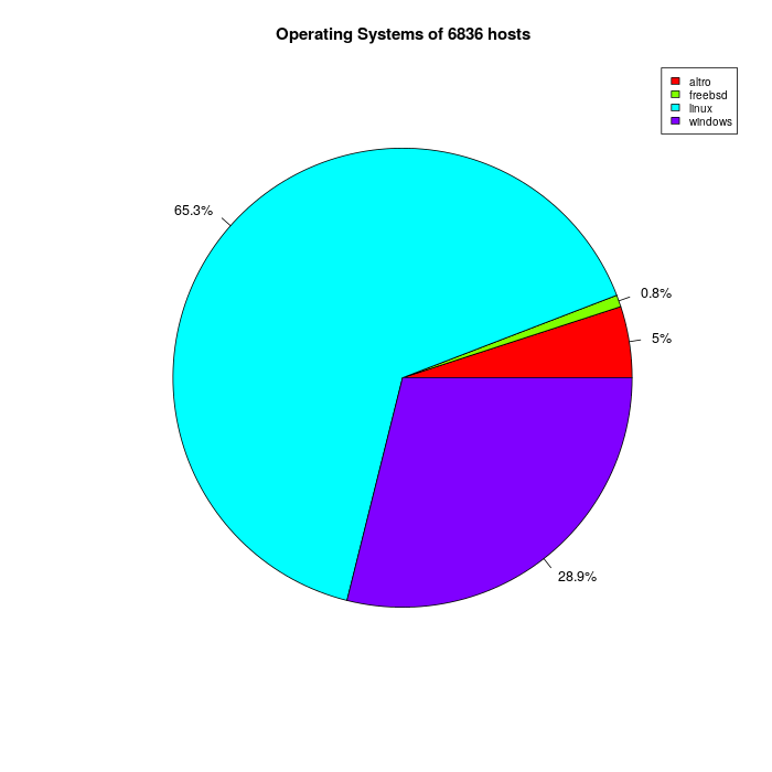
Operating Systems
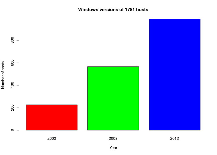
Versions of Windows
Versions of Linux
Types of CMS
Types of Server on port 80
Versions of the most Server used
Types of Server on port 443
Presence of SSL
HeartBleed
As you can see, there are a lot of outdated services. The most relevant data are:
- 65% of websites don’t have any SSL certificate;
- 27% of websites still vulnerable to Heartbleed;
- More than 200 websites use Windows Server 2003;
- More than 500 different types of Hosting on 7000 sites;
Perhaps the government should invest on information security, rather than design.